Import Global SRTM Elevation Data Into Postgres Database Using PostGIS

Sam Chance

August 6, 2024

TLDR

In this article, we walk through the process of obtaining and downloading rasters of global digital elevation data from the SRTM satellite.

We split these rasters into tiles and import them into a local Postgres database using PostGIS.

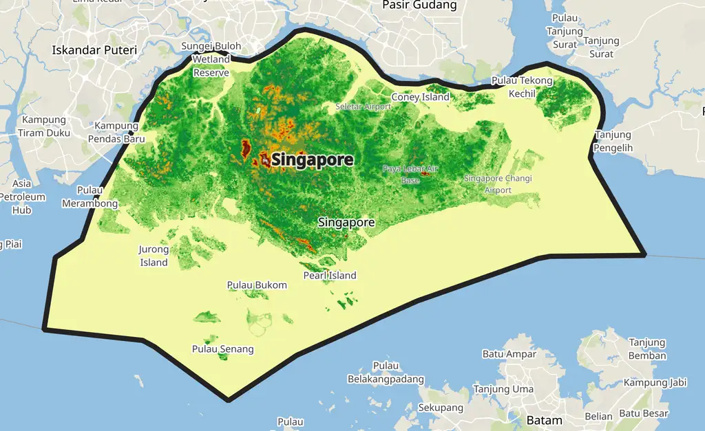
We then use tiles from this database to construct a query using PostGIS functions to generate a single DEM raster of Singapore and import this into QGIS.

The final image looks like this:

Introduction

It’s possible to download the entire SRTM (Shuttle Radar Topography Mission) satellite imagery dataset and insert it into a Postgres database for personal use. This can be helpful for if you need global elevation data for your analysis and don’t want to be limited by third-parties APIs.

The SRTM is a near-global dataset of elevation data with a resolution of 1-arc-second (30m). More information is available from USGS. In this guide we will go through the process of downloading the data, inserting it into a Postgres database with PostGIS, then querying the final result to create a DEM for any country or region.

This guide assumes you are using Linux (this may also apply to other Unix like systems such as MacOS) and have a Postgres database with the PostGIS extension installed. More information on how to do this can be found on the PostGIS website.

Download data

We’ll download the data from the OpenTopography AWS S3 bucket. You should create a free account with them before downloading. Also, remember to provide citations where necessary.

To download the data, first we need to install the AWS CLI utility:

# install for linux
curl "https://awscli.amazonaws.com/awscli-exe-linux-x86_64.zip" -o "awscliv2.zip"
unzip awscliv2.zip
sudo ./aws/install

# MacOS
curl "https://awscli.amazonaws.com/AWSCLIV2.pkg" -o "AWSCLIV2.pkg"
sudo installer -pkg AWSCLIV2.pkg -target /

Next we can run the following command to download the rasters. This will take some time depending on your internet speed. The final size is about 127GB and took me about 1 hour to download on a 600MB connection.

aws s3 cp s3://raster/SRTM_GL1/ . --recursive --endpoint-url https://opentopography.s3.sdsc.edu --no-sign-request

If you’d prefer to download specific rasters or rasters for a region instead of downloading them all, you can select regions for download from the OpenTopography website using the interactive map.

Using raster2pgsql to import raster tiles into PostGIS

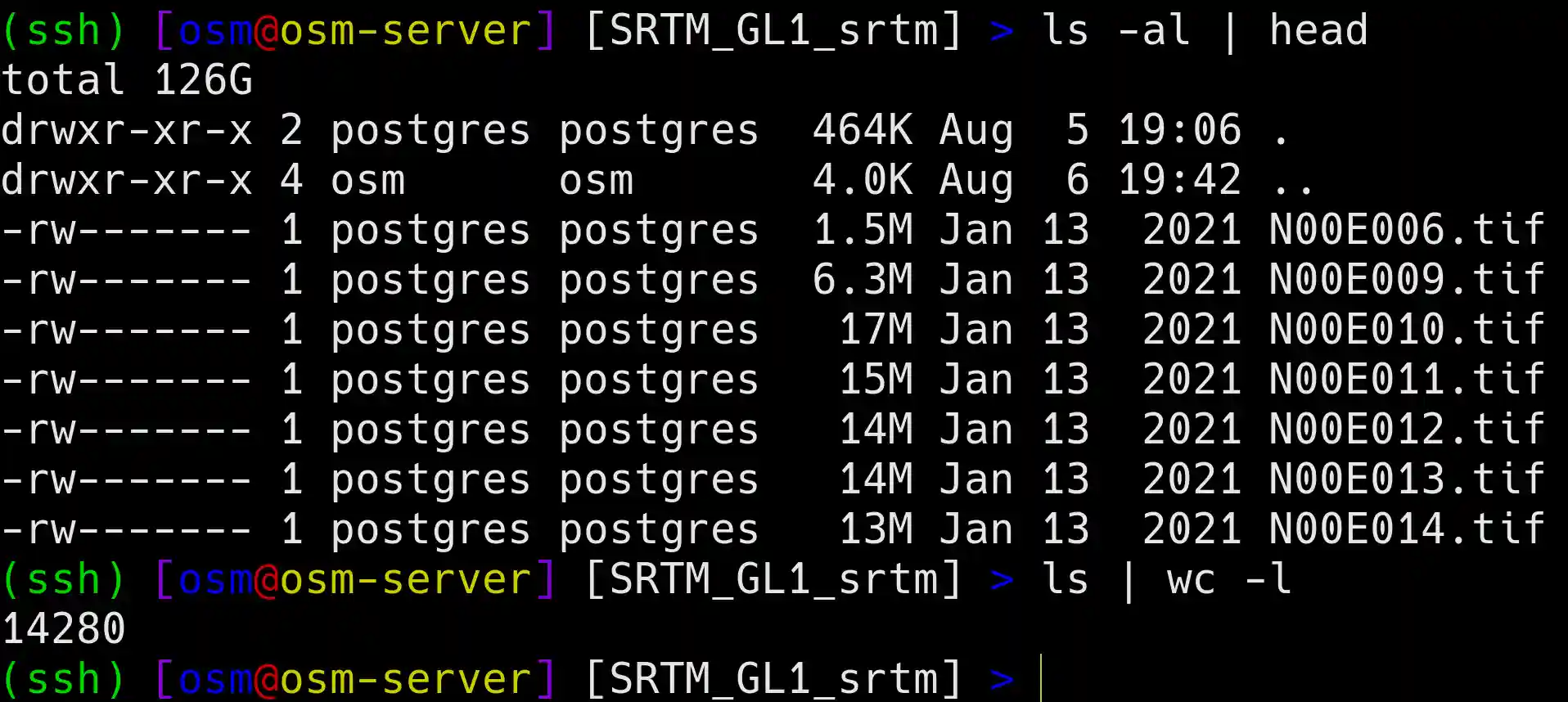
Now we have the data downloaded on our system, we can import it into our database. If we look inside the SRTM_GL1_srtm directory, we can see all of the 14280 raster files:

Next we will use the raster2pgsql command to import these rasters into our database.

raster2pgsql -d -M -C -I -s 4326 -t 128x128 -F *.tif dem.srtm | psql --dbname=osm --username=postgres -h 127.0.0.1

Here’s a breakdown of the above command:

-d This drops an existing table if it already exists. It’s useful to include this in case we need to run the command again.
-M This runs VACUUM ANALYZE on the table after the raster tiles have been inserted into the database. This optimizes the table by reclaiming storage space and then collecting table statistics.
-C This applies raster constraints to the table by using the AddRasterConstraints function in PostGIS. This adds several types of constraints to the table which ensures data integrity and enforces rules for consistency.
-I Creates a spatial index (GiST) on the table.
-s Assign SRID (Spatial Reference System Identifier) to the raster.
-t Tile size. This splits the raster into tiles of the specified size. Each tile is a row in the final table.
-F Creates a filename column. As the raster is split into many smaller tiles, this is useful to help us identify the original file the tile belonged to.
*.tif Selects all of the .tif files in the directory.
dem.srtm Defines the schema and name of the table. Remember to create the dem schema in the database before running the command.

The raster2pgsql command will output a sql query which we can then pipe into the psql command.

For more information on the raster2pgsql command, please visit the PostGIS website.

This process will take a couple of hours. It could take longer if running over a network, so it’d be best to run this command on the same machine as the Postgres instance.

Once this process has completed, we can query the table to see how many tiles we have:

select count(*) from dem.srtm

  count  
---------
 12009480

So we have just over 12 million 128x128 tiles in the database.

Raster Clipping

Now we have global SRTM data loaded in our local database, we can extract the tiles we want for further analysis.

Here we’ll create a digital elevation raster for Singapore to demonstrate using the following PostGIS commands: st_clip, st_intersects and st_union, then import this into QGIS to style and visualise the results.

I already have countries vector data in my Postgres database that I extracted from OpenStreetMaps. You can download a pg_dump of this here to insert into your database. Alternatively, I have a post here that explains the process to do this manually.

To create our table, we’ll use the following SQL. I’ll break down each section step-by-step.

First we’ll use the st_intersects command to select all of the raster tiles that intersect with the Singapore polygon. Note, we’ll need to create a table, spatial index then apply constraints for this to work in QGIS.

-- drop existing table and create a new table
drop table if exists dem.singapore_srtm;
create table dem.singapore_srtm as

-- cte to create polygon of singapore
with country as (select geom as geom from dev.countries where country = 'Singapore')

-- select tiles that intersect with the Singapore polygon using a left join and st_intersects function
select srtm.rast, srtm.rid
from dem.srtm srtm
join country ply on st_intersects(ply.geom, st_convexhull(srtm.rast));

-- create index and apply constraints
create index on "dem"."singapore_srtm" using gist (st_convexhull("rast"));
analyze "dem"."singapore_srtm" ;
select addrasterconstraints( 'dem', 'singapore_srtm', 'rast', true, true, true, true, true, true, false, true, true, true, true, true) ;

Now we can query the table:

-- check number of tiles in the table
select count(*) from dem.singapore_srtm

 count 
-------
   153

Here we have 153 of our 128x128 tiles.

We can visualise these tiles in QGIS: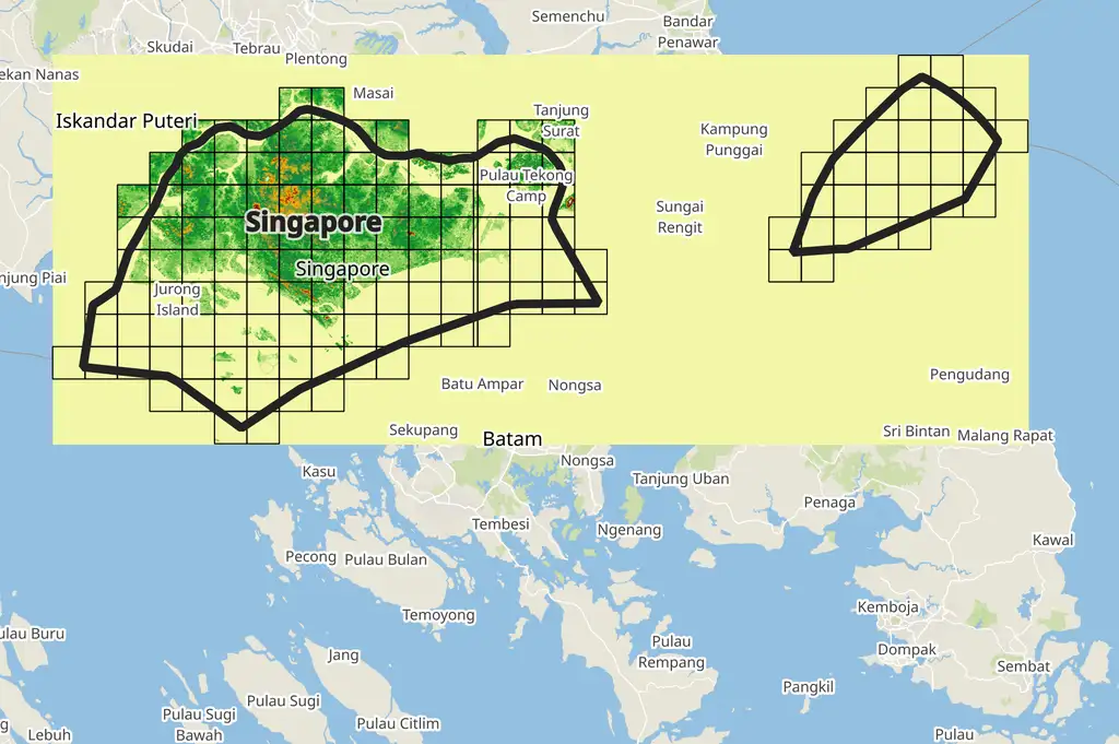

Note, you can use the st_convexhull command to generate an outline of the raster tiles as seen in the previous figure:

select row_number() over () as uid, st_convexhull(rast) as geom
from dem.singapore_srtm

It would be nice to remove the pixels outside of the Singapore polygon. For this we can use the st_clip function along with st_intersect:

-- drop existing table and create a new table
drop table if exists dem.singapore_srtm;
create table dem.singapore_srtm as

-- cte to create polygon of singapore
with country as (select geom as geom from dev.countries where country = 'Singapore'),

-- cte to clip tiles to the singapore polygon
clipped_tiles as (
select st_clip(srtm.rast, ply.geom, true) as rast, srtm.rid
from dem.srtm srtm
join country ply on st_intersects(ply.geom, st_convexhull(srtm.rast))
)

select rast as rast
from clipped_tiles;

-- create index and apply constraints
create index on "dem"."singapore_srtm" using gist (st_convexhull("rast"));
analyze "dem"."singapore_srtm" ;
select addrasterconstraints( 'dem', 'singapore_srtm', 'rast', true, true, true, true, true, true, false, true, true, true, true, true) ;
vacuum analyze "dem"."singapore_srtm";

Give us this:

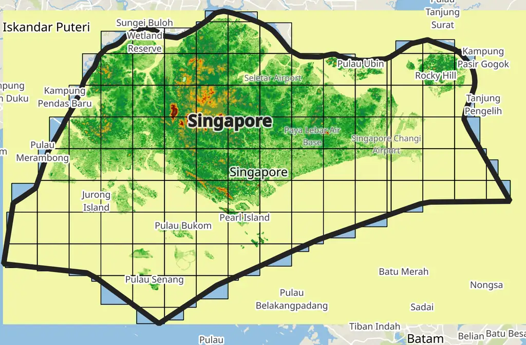
Hmm, this doesn’t look quite right! As you can see, the clipped tiles only seem to apply within the tile boundaries outside of the clip region. These areas have been set to nodata (which is expected). However, outside of that, QGIS is rendering those pixels as something else (it’s rendering them as having a value of 0).

The reason for this is because we are not strictly importing a single raster into QGIS, rather we are still importing all of the indivitual tiles. Since GeoTIFFs are rasters that can only exist as a grid of pixels (i.e. a rectangle), QGIS must therefore render the entire raster extent, which leads to the unusual rendering issue above.

We can solve this by using the st_union function in our query. This takes all of the individual raster tiles and unions them into a single raster. All of the nodata values for the extent of the clipped region will also be unioned, thus creating a single rectangular raster that we can import into QGIS.

Our final query will look like this:

-- drop existing table and create a new table
drop table if exists dem.singapore_srtm;
create table dem.singapore_srtm as

-- cte to create polygon of singapore
with country as (select geom as geom from dev.countries where country = 'Singapore'),

-- cte to clip tiles to the singapore polygon
clipped_tiles as (
select st_clip(srtm.rast, ply.geom, true) as rast, srtm.rid
from dem.srtm srtm
join country ply on st_intersects(ply.geom, st_convexhull(srtm.rast))
)

-- union tiles into a single raster
select st_union(rast) as rast
from clipped_tiles;

-- create index and apply constraints
create index on "dem"."singapore_srtm" using gist (st_convexhull("rast"));
analyze "dem"."singapore_srtm" ;
select addrasterconstraints( 'dem', 'singapore_srtm', 'rast', true, true, true, true, true, true, false, true, true, true, true, true) ;
vacuum analyze "dem"."singapore_srtm";

Looks much better!

This DEM raster of Singapore is available for download from the downloads page here

Citations

NASA Shuttle Radar Topography Mission (SRTM)(2013). Shuttle Radar Topography Mission (SRTM) Global. Distributed by OpenTopography. https://doi.org/10.5069/G9445JDF. Accessed: 2024-08-06